Making a model

As illustrated in the architecture page, SATLAS2 is built on the concept of a Fitter object, to which Source objects are assigned. These Source objects contain both experimental data, but are also assigned one or more Models, which should be fitted to the data.

The base aspect of these Models is that two things should be implemented: a params attribute which is a dictionary containing all the Parameters that the Model needs, and a method f(x), where the response for the given x values is returned. It is recommended that the first line of the method is x = self.transform(x) in order to correctly handle any transformation functions that are required.

In this tutorial, a new Model will be created to model a sine wave with exponential damping called ExpSine, just as an example. In the preamble, we just import all the libraries that we will need.

import sys

sys.path.insert(0, '..\src')
import matplotlib.pyplot as plt
import numpy as np

import satlas2

Subclassing Model

The new class will be a subclass of the SATLAS2 Model class, and it will contain SATLAS2 Parameters in its params dictionary.

class ExpSine(satlas2.Model):
    def __init__(self, A, lamda, omega, name='ExpSine', prefunc=None):
        super().__init__(name, prefunc=prefunc)
        self.params={
            'amplitude': satlas2.Parameter(value=A,min=0,max=np.inf,vary=True),
            'lambda': satlas2.Parameter(value=lamda, min=0, max=np.inf, vary=True),
            'omega': satlas2.Parameter(value=omega, min=0, max=np.inf, vary=True)
        }

    def f(self, x):
        x = self.transform(x)
        a = self.params['amplitude'].value
        l = self.params['lambda'].value
        o = self.params['omega'].value
        return a*np.exp(-l*x)*np.sin(o*x)

This defines a sine wave of angular frequency ω with an exponential decay with decay constant λ. Note that, in the parameter name in init, lamda is used instead of lambda since the last one is a keyword in Python.

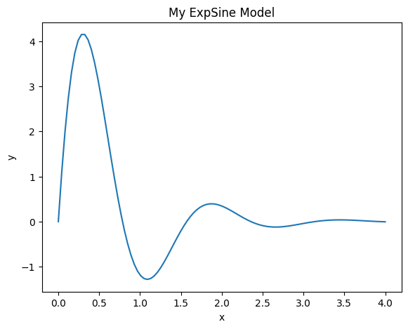
With this new Model, plotting is done in the following way:

amplitude = 7
lamda = 1.5
omega = 4
model = ExpSine(amplitude, lamda, omega, name='MyModel')

x = np.linspace(0, 4, 100)
y = model.f(x)

fig = plt.figure()
ax = fig.add_axes([0.1, 0.1, 0.8, 0.8])
ax.plot(x, y)
ax.set_xlabel('x')
ax.set_ylabel('y')
ax.set_title('My ExpSine Model')
model.params

{'amplitude': 7+/-0 (inf max, 0 min, vary=True, correl={}),
 'lambda': 1.5+/-0 (inf max, 0 min, vary=True, correl={}),
 'omega': 4+/-0 (inf max, 0 min, vary=True, correl={})}

Data generation and fitting

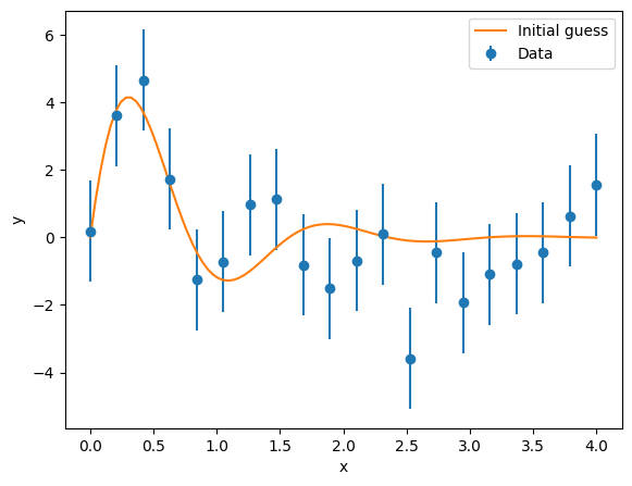
The model defined above is fully compatible with all SATLAS2 code and can be used to fit data. To illustrate this feature, a dataset needs to be generated. For this, SATLAS2 contains a convenience function. The standard argument generates a dataset that assumes the model supplies the mean value of a Poisson distribution, which is useful for simulation of laser spectroscopy spectra. However, the generator can be modified, allowing generic Gaussian data to be generated as well:

data_x = np.linspace(0, 4, 20)
noise = 1.5
generator = lambda x: np.random.default_rng(0).normal(x, noise)
data_y = satlas2.generateSpectrum(model, data_x, generator=generator)
yerr = np.ones(data_y.shape)*noise

fig = plt.figure()
ax = fig.add_axes([0.1, 0.1, 0.8, 0.8])
ax.errorbar(data_x, data_y, yerr=yerr, fmt='o', label='Data')
ax.plot(x, y, label='Initial guess')
ax.set_xlabel('x')
ax.set_ylabel('y')
ax.legend(loc=0)

We assign this data to a Source, add the ExpSine model to this Source, and pass it to a Fitter to fit this. Since this requires a normal chisquare fit, no extra arguments are required for the fit.

datasource = satlas2.Source(data_x, data_y, yerr=yerr, name='Datafile1')
datasource.addModel(model)
f = satlas2.Fitter()
f.addSource(datasource)
f.fit()
print(f.reportFit())
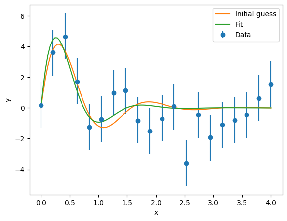
fig = plt.figure()
ax = fig.add_axes([0.1, 0.1, 0.8, 0.8])
ax.errorbar(data_x, data_y, yerr=yerr, fmt='o', label='Data')
ax.plot(x, y, label='Initial guess')
ax.plot(x, model.f(x), label='Fit')
ax.set_xlabel('x')
ax.set_ylabel('y')
ax.legend(loc=0)

[[Fit Statistics]]
    # fitting method   = leastsq
    # function evals   = 93
    # data points      = 20
    # variables        = 3
    chi-square         = 14.1735643
    reduced chi-square = 0.83373907
    Akaike info crit   = -0.88707432
    Bayesian info crit = 2.10012250
[[Variables]]
    Datafile1___MyModel___amplitude:  9.03884096 +/- 4.31842559 (47.78%) (init = 7)
    Datafile1___MyModel___lambda:     2.15722712 +/- 1.22083220 (56.59%) (init = 1.5)
    Datafile1___MyModel___omega:      4.22415871 +/- 0.68336353 (16.18%) (init = 4)